Start of topic | Skip to actions
3D Euler equations - Forward facing step
3 Grid Levels (time t = 4.0)
Results:
| Level 0 | Level 1 | Level 2 | |
| Grids | 23 | 27 | 427 |
| Cells | 43392 | 320256 | 1395752 |
Color, schlieren and contour plots of the density (click on pictures to display cuts!)
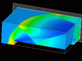 | 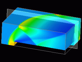 | |
| cuttig plane at z=2.0 | cutting plane at z=1.2 | |
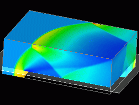 | 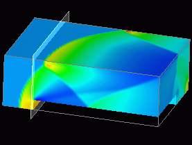 | |
| cutting plane at y=0.2 | cutting plane at x=0.6 |
Distribution to 4 processors (back left view)
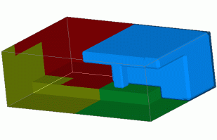 | 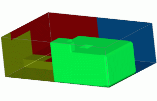 | |
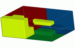 | 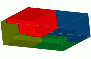 |
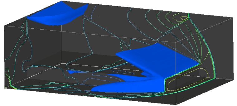
Regions of low density (back left view, iso surface at density=0.92)
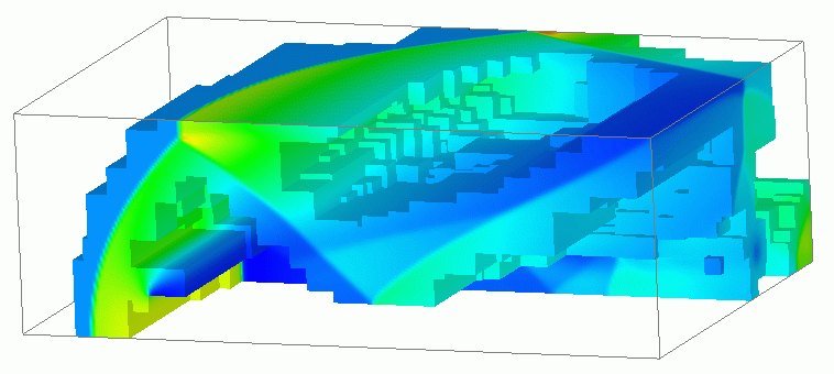
Blocks of the second refinement level (front right view)
Benchmark
| Task | P=1 | P=2 | P=4 | |||
| s | % | s | % | s | % | |
| Integration | 160927 | 39.6 | 40695 | 49.9 | 18583 | 45.5 |
| Flux correction | 23030 | 5.7 | 1516 | 1.9 | 1361 | 3.3 |
| Boundary setting | 68094 | 16.7 | 19092 | 23.4 | 12921 | 31.6 |
| Recomposition | 118589 | 29.2 | 13540 | 16.6 | 5748 | 14.1 |
| Clustering | 10790 | 2.7 | 2100 | 2.6 | 577 | 1.4 |
| Misc. | 25113 | 6.2 | 4560 | 5.6 | 1653 | 4.1 |
| Total / parall. efficiency | 406543 | 100.0 | 81503 | 249.4 | 40843 | 248.8 |
|---|---|---|---|---|---|---|
<--- Problem description
-- RalfDeiterding - 06 Dec 2004