2D Euler equations - Explosion in a Box

Variation of Distribution (situation at time t=0.5)

Results: 2 Levels / 3 Levels / Variation of Distribution / Variation of GuC-Factor

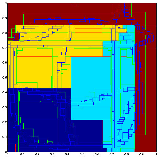
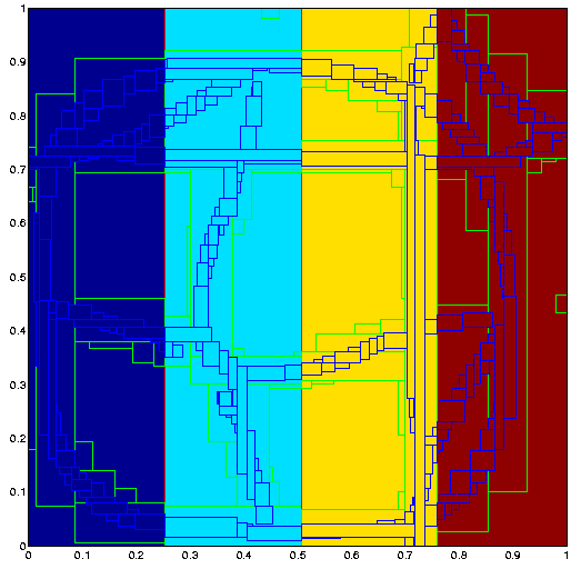
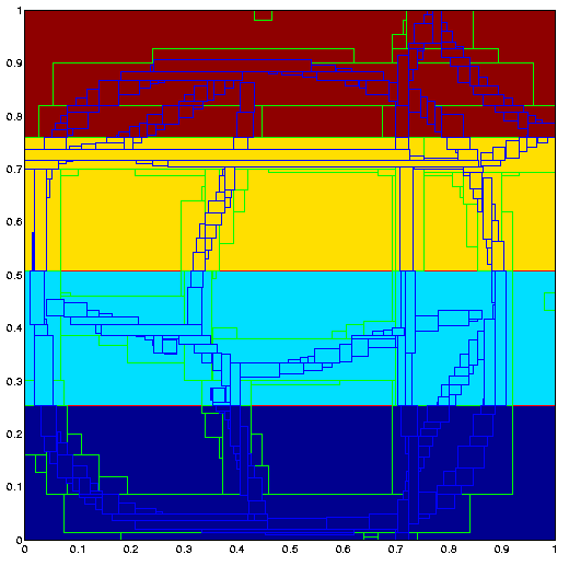
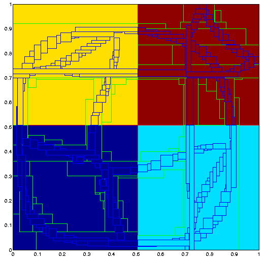
Beside the Hilbert space-filling curve a fixed regular distribution can be chosen. For this particular example, the Hilbert space-filling curve and the regular XY-distribution lead to comparable computational times.

Workload for different distribution types. 4 computing nodes are used.

Distribution	P1	P2	P3	P4
Hilbert	0.932	1.062	1.044	0.962
X	0.937	1.084	0.999	0.980
Y	0.941	1.079	1.004	0.976
XY	0.982	1.037	1.030	0.950

Distribution with Hilbert space filling curve, Distribution=1

Distribution in x-direction, Distribution=2

Distribution in y-direction, Distribution=3

Distribution in xy-direction, Distribution=5

---

Benchmark

Task	Hilbert		X		Y		XY
	s	%	s	%	s	%	s	%
Integration	2246	67.2	3243	72.0	3230	71.9	2676	71.7
Flux correction	180	5.4	283	6.3	281	6.3	132	3.5
Boundary setting	315	9.4	171	3.8	164	3.6	134	3.6
Recomposition	496	14.9	676	15.0	686	15.3	678	18.2
Clustering	37	1.1	51	1.1	51	1.1	43	1.2
Misc.	56	2.0	70	1.8	72	1.8	61	1.9
Total / Parallel Efficiency	3329	85.1	4495	63.0	4485	63.2	3584	79.1

P=4, GuC-Factor=2

<--- Problem description

---

-- RalfDeiterding - 04 Dec 2004